Essentials of Data Science – Probability and Statistical Inference - Normal Distribution

In this note series on Probability and Statistical Inference, we have already seen the importance of probability distributions and their associated probability functions for discrete random variables. In addition, we have learned to resemble a natural random phenomenon with these probability distributions. These distributions were Degenerate distribution, Uniform distribution, Bernoulli distribution, Binomial distribution, Poisson distribution, and Geometric distribution.

This note will cover probability distributions and their associated probability functions for continuous random variables. We have already covered Continuous Uniform Distribution, and now we will explore Normal Distribution, a most widely used probability density function to model the random phenomenons. It has enormous applications in Data Science.

Table of Contents hide

1 Normal Distribution

1.1 Properties of Normal Distribution

1.2 Cumulative Distribution Function

2 Standard Normal Distribution

2.1 Z Transformation

3 Normal Distribution – Examples

3.1 Sample Random Variables from Normal Distributution

4 References

4.1 Share this:

4.2 Like this:

Normal Distribution

The normal distribution is one of the essential distributions used in statistics. It is also called Gaussian distribution. The most widely used model for the distribution of a random variable is a normal distribution.

A random variable X is said to follow a normal distribution with parameters $\mu$ and $\sigma^2$ if its Probability Density Function (PDF) is given by:

$f(x; \mu, \sigma^2) \sim f(x) = \frac{1}{\sigma \sqrt{2 \pi}} e^{- \frac{(x - \mu)^2}{2 \sigma^2}}$ , $- \infty < x < \infty; -\infty < \mu < \infty; \sigma^2 > 0$

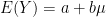
The mean and variance of X are:

$E(X) = \mu$
$Var(X) = \sigma^2$

The value of E(X) determines the centre of the probability density function, and the value of Var(X) determines the width. It is also represented as $N(\mu,\sigma^2)$ .

Properties of Normal Distribution

The density of normal distribution has its maximum at $x = \mu$ .
The density of the curve is symmetric and bell-shaped.
The inflexion points of the density are at $(\mu - \sigma)$ and $(\mu + \sigma)$

A lower $\sigma$ indicates a higher concentration around the mean $\mu$ . It means lower variance and data is concentrated towards the mean.
A higher $\sigma$ indicates a flatter density. It means higher variance and data points are distributed across the distribution.

Normal distribution - Mean and Variance — Normal distribution – Mean and Variance

Two normal distributions having the same mean value do not tell about the variance, and similarly, having the same variance of two normal distributions does not speak about mean values. These two characteristics are different and represent two different properties of a density curve.

Normal distribution probabilities are associated with the 68-95-99.7 rule. It means, 68% of the data is within one standard deviation $\sigma$ of the mean $\mu$ . Similarly, 95% of the data is within two standard deviation $\sigma$ of the mean $\mu$ and 99.7% of the data is within three standard deviation $\sigma$ of the mean $\mu$ .

Cumulative Distribution Function

The cumulative distribution function of $X \sim N(\mu, \sigma^2)$ is:

$F(x) = \int_{- \infty}^{x} \phi(t) dt$

which is often denoted as $\Phi(x)$ .

There is no explicit formula to solve the integral. It has to be solved by numerical or computational methods. This is why CDF tables are presented in almost all statistical textbooks.

Standard Normal Distribution

If $\mu = 0$ and $\sigma^2 = 1$ , then X is said to follow a standard normal distribution. The PDF of a standard normal distribution is given by:

$f(x) = \frac{1}{\sigma \sqrt{2 \pi}} e^{- \frac{x^2}{2}}$ , $- \infty < x < \infty;$

Important results:

If X is normally distributed with mean $\mu$ and variance $\sigma^2$ , then for any constants a and b != 0, the random variable Y which is equal to Y = a + bX is also a normally distributed with parameters as follows:

$E(Y) = a + b \mu$
$Var(Y) = b^2 Var(X) = b^2 \sigma^2$

If X is normally distributed with mean $\mu$ and variance $\sigma^2$ , let Z is another random variable as follows:

$Z = \frac{X - \mu}{\sigma}$ ,

$E(Z) = \frac{E(X - \mu)}{\sigma} = \frac{E(X) - \mu}{\sigma} = 0$
$Var(Z) = \frac{Var(X)}{\sigma^2} = \frac{\sigma^2}{\sigma^2} = 1$

It has a standard normal distribution N(0,1) called a Z transformation. This result helps us to find different probability statements about X in terms of probabilities for Z. In simple words; a normally distributed random variable becomes a standard normal distributed random variable when we perform Z transformation.

Z Transformation

It is a process of standardization that allows for the comparison of scores from disparate distributions. Using a distribution’s mean and standard deviation, z transformations convert separate distributions into a standardized distribution, allowing for the comparison of dissimilar metrics.

The standardized distribution is made up of z scores, hence the term z transformation.
Z scores are a special type of standard score in which each unit represents one standard deviation from the mean.
Z scores always have a distribution with a mean value of 0 and a standard deviation of 1.

Important results:

If X is standard normal distribution with mean $\mu$ and variance $\sigma^2$ , then Cumulative Distribution Function (CDF) $\Phi$ can be computed as follows:

Analysis of Normal Distribution — CDF of Normal Distribution

After Z transformation, finding CDF becomes easy as $\mu = 0$

(mean) and $\sigma^2 = 1$

(variance) values are fixed and the below equations illustrated these things.

$\Phi(z) = \int_{- \infty}^{z} \phi(t) dt$ where $\phi$ is the pdf of $N(\mu,\sigma^2)$
$\Phi(-z) = 1 - \Phi(z)$
$\Phi(-z) + \Phi(z) = 1$ , total area under the whole curve is 1.
$\Phi(0) = \frac{1}{2}$

Normal Distribution – Examples

Example 1: An apple farmer sells the apples in boxes. The weights of the boxes vary and are assumed to be normally distributed with $\mu$ = 20 kg and $\sigma^2 = 2 \text{kg}^2$ . The farmer wants to avoid customers being unsatisfied because the boxes are too low in weight.

Therefore the farmer wants to know the probability that a box with a weight of less than 18 kg is sold.

Solution: This can be obtained by computing $P(X \leq 18)$ = 0.158

from scipy.stats import norm
norm(loc=20,scale=2).cdf(18)

which is equal to 15%.

Sample Random Variables from Normal Distributution

Consider a random sample $X = X_1, X_2, \cdots, X_n$ and these independent and identically distributed random variables $X_i$ with $X_i \approx N(\mu,\sigma^2)$ distribution. Then,

Arithmetic mean:

$\bar{X}$ = $\frac{1}{n} \sum_{i=1}^n X_i \approx N \left ( \mu, \frac{\sigma^2}{n}\right)$

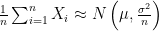
Expectation:

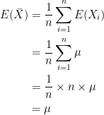
$\begin{aligned} E(\bar{X}) &= \frac{1}{n} \sum_{i=1}^n E(X_i) \\ &= \frac{1}{n} \sum_{i=1}^n \mu \\ &= \frac{1}{n} \times n \times \mu \\ &= \mu \end{aligned}$

Variance:

$\begin{aligned} Var(\bar{X}) &= \frac{1}{n^2} \sum_{i=1}^n Var(X_i) \\ &= \frac{1}{n^2} \sum_{i=1}^n \sigma^2 \\ &= \frac{1}{n^2} \times n \times \sigma^2 \\ &= \frac{\sigma^2}{n} \end{aligned}$

where $\text{ Cov}(X_i,X_j) = 0 \text{ for } i \neq j$

References

Essentials of Data Science With R Software – 1: Probability and Statistical Inference, By Prof. Shalabh, Dept. of Mathematics and Statistics, IIT Kanpur.

CITE THIS AS:

“Probability and Statistical Inference – Introduction to Normal Distribution” From NotePub.io – Publish & Share Note! https://notepub.io/notes/mathematics/statistics/statistical-inference-for-data-science/normal-distribution/

22,593 total views, 1 views today

Essentials of Data Science – Probability and Statistical Inference – Normal Distribution