In the previous note on discrete random variables, we have seen what a discrete random variable is and its distribution function. In the case of a discrete random variable, the distribution function is expressed in terms of probability mass function (PDF) and cumulative distribution function (CDF).
In this note, we will further extend the concept of the random variables and explore what an expectation is and how to compute for discrete and continuous random variables.
Introduction
Let us understand what an expectation is. Suppose two participants are playing a coin-tossing game, assume that coin is fair and chances of getting head and tail are equally likely, as well as same rewards for winner or loser.
- Case 1: The outcome will be equally likely to gain or lose in the game if we do the mental calculation.
- Case 2: If we change the reward proportion, let’s say, X amount needs to be paid by the first participant when they lose and receive 2X amount when they win. It is a special offer for the first participant. Although the first participant knows that winning or losing chances are equally likely, the expected chances of success are higher due to changes in reward proportion. Moreover, indirectly the first participant does mental calculations and figures out that the average or expected success rate is higher than failure in the game.
This is how we always compute the average or expected value for grabbing or passing the opportunities in every perspective of our life, which means we know how to calculate the expected value from the observations.
Now, we will try to understand what does expectation mean using the same example, but in more mathematical way.
Example 1:
Suppose we toss a coin, assume that coin is fair and chances of getting head and tail are equally likely. The possible outcomes are head and tail, {H,T}. The reward formulation are as follows:
- If we get head, we get a reward of Rs. 2.
- If we get tail, we get a reward of Rs. 4.
What do we expect to get an average reward ?
- P(H) = P(T) = 1/2
- Expected average reward = Rs. 2 * P(H) + Rs. 4 * P(T) = 2 * 1/2 + 4 * 1/2 = Rs. 3
Example 2:
Suppose we roll a dice and rewards are considered in the following ways:
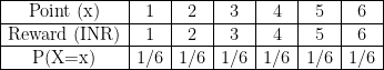
In this example, Point(x) represents a number that appears on the upper face of the die, and Reward (INR) represents rewards for different values of x. However, each outcome’s probabilities are equally likely, which means anyone occurs with the same probability.
The expected reward means when we play this game a significantly higher number of times, the accumulated rewards would be equal to the expected reward value.
Expected reward: Rs. 1 * 1/6 + Rs. 2 * 1/6 + Rs. 3 * 1/6 + Rs. 4 * 1/6 + Rs. 5 * 1/6 + Rs. 6 * 1/6 = Rs. 3.50
Expectation of a Continuous Random Variable
Let X be a continuous random variable having the probability density function f(x). Suppose g(X) is a real valued function of X. The expectation of g(X) is defined as:
![E[g(X)] = \int_{-\infty}^{\infty} g(x)f(x) dx](https://s0.wp.com/latex.php?latex=E%5Bg%28X%29%5D+%3D+%5Cint_%7B-%5Cinfty%7D%5E%7B%5Cinfty%7D+g%28x%29f%28x%29+dx&bg=ffffff&fg=000&s=0&c=20201002)

Example 1: Consider the continuous random variable “waiting time for the train”. Suppose that a train arrives every 20 min. Therefore, the waiting time of a particular person is random and can be any time contained in the interval [0,20].
The required probability density function is

Solution:

Thus the average waiting time for the train is 10 minutes, which means that if a person has to wait for the train every day, then the waiting time will vary randomly between 0 and 20 minutes and, avarage it will be 10 minutes.
Expectation of a Discrete Random Variable
Let X be a discrete random variable having the probability mass function 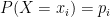


![E[g(X)] = \sum_{i=1}^{\infty} g(x_i)P(X=x_i) = \sum_{i=1}^{\infty} g(x_i)p_i](https://s0.wp.com/latex.php?latex=E%5Bg%28X%29%5D+%3D+%5Csum_%7Bi%3D1%7D%5E%7B%5Cinfty%7D+g%28x_i%29P%28X%3Dx_i%29+%3D+%5Csum_%7Bi%3D1%7D%5E%7B%5Cinfty%7D+g%28x_i%29p_i&bg=ffffff&fg=000&s=0&c=20201002)

Example 1: Suppose we roll a dice and following is the scheme for award based on outcomes.
The required probability mass function is:

Solution:
![\begin{aligned} E[X] &= \sum_{i=1}^{\infty} g(x_i) \times P(X=x_i) \\ &= \sum_{i=1}^{6} g(x_i)p_i \\ &= 1 \times 1/6 + 2 \times 1/6 + 3 \times 1/6 + 4 \times 1/6 + 5 \times 1/6 + 6 \times 1/6 \\ & = Rs. 3.5 \end{aligned}](https://s0.wp.com/latex.php?latex=%5Cbegin%7Baligned%7D+E%5BX%5D+%26%3D+%5Csum_%7Bi%3D1%7D%5E%7B%5Cinfty%7D+g%28x_i%29+%5Ctimes+P%28X%3Dx_i%29+%5C%5C+%26%3D+%5Csum_%7Bi%3D1%7D%5E%7B6%7D+g%28x_i%29p_i+%5C%5C+%26%3D+1+%5Ctimes+1%2F6+%2B+2+%5Ctimes+1%2F6+%2B+3+%5Ctimes+1%2F6+%2B+4+%5Ctimes+1%2F6+%2B+5+%5Ctimes+1%2F6+%2B+6+%5Ctimes+1%2F6+%5C%5C+%26+%3D+Rs.+3.5+%5Cend%7Baligned%7D&bg=ffffff&fg=000&s=0&c=20201002)
Special Cases of Expectation of a Random Variable
Case1: g(X) = X then E[g(X)] = E(X). The expectation of X, i.e. E(X), is ususally denoted by 
Case2: If a and b are any real constants, then E(a) = a and E[aX + b] = aE(X) + b
Case3: Let 

![E[\sum_{1=1}^r g_i(X)] = \sum_{i=1}^r E[g(X_i)]](https://s0.wp.com/latex.php?latex=E%5B%5Csum_%7B1%3D1%7D%5Er+g_i%28X%29%5D+%3D+%5Csum_%7Bi%3D1%7D%5Er+E%5Bg%28X_i%29%5D&bg=ffffff&fg=000&s=0&c=20201002)
Summary
Probability Space
We have seen what an experiment is and the possible outcomes of the experiments. Based on the experiment’s outcomes, we can decide whether random variables would be discrete and continuous. The definition of the random variable is entirely dependent on the experiment goal. However, it should satisfy the random variable criteria.
Once we have a random variable and associated distribution function, we can calculate probabilities at a point and probability area under the curve, in the case of a discrete random variable and continuous random variable, respectively. These values can be stored in a tabular fashion or we can say that values of the probability function of a random variable.
Statistical Space
From the distribution data, we can learn various parameters that may help to understand the characteristics of an experiment based on our interest which is defined using a random variable. The characteristics could be the central tendency, data dispersion, skewness, kurtosis, correlation coefficient, etc. We always represent data based on these characteristics because it is impossible to talk about individual data points, which may not give relevant information to make statistical decisions.
It shows how we have shifted our random experiment model from probability to statistical space to derive meaning information from the results.
References
- Essentials of Data Science With R Software – 1: Probability and Statistical Inference, By Prof. Shalabh, Dept. of Mathematics and Statistics, IIT Kanpur.
CITE THIS AS:
“Expectation of Variables” From NotePub.io – Publish & Share Note! https://notepub.io/notes/mathematics/statistics/statistical-inference-for-data-science/expectation-of-variables/
65,440 total views, 1 views today