In the previous note on Probability and Statistical Inference, we have seen the importance of probability distributions.
This note will cover the basic intuition behind Bernoulli and Binomial distributions, expectation, variance, and other quantitative measures to characterize the probability distribution. Further, we will also cover various similar phenomena following Bernoulli and Binomial distributions.
Using the probability functions of Bernoulli and Binomial distributions, we can compute expectation, variance, and other quantitative measures of similar phenomenons.
Bernoulli Distribution
A Bernoulli experiment is a random experiment, the outcome of which can be classified in one of two mutually exclusive and exhaustive ways, e.g., success or failure; female or male; life or death; non-defective or defective.
- Mutually exclusive means, both can’t occur at the same time. However, there is no guarantee that one of the events will occur.
- Mutually exhaustive means, one of them must occur.
In contrast, degenerate distribution indicates that there is only one possible fixed outcome, and therefore, no randomness is involved. We need at least two different possible outcomes to have randomness in the observations of a random variable or random experiment.
Bernoulli distribution is useful when there are only two possible outcomes, and our interest lies in any of the two outcomes. Moreover, these outcomes are usually denoted by the values zero and one. For example:
- Whether a customer buys a certain product or not.
- Whether a student will clear the entrance examination or not.
Suppose X is a random variable, and it takes two values, zero and one. Let X = 1 when the outcome is a success and X = 0 when the outcome is a failure. A random variable X has a Bernoulli distribution if the probability mass function of X is given as follows:

The CDF in such a case is given by

The mean (expectation) and variance of a Bernoulli random variable are calculated as follows:
- E(X) = p
- Var(X) = p(1-p)
Example 1: There are 300 lottery tickets in total, and 50 of them are marked as winning tickets.
Suppose an event A of interest is ticket wins ( Let us consider X = 1), and the probability p of having a winning ticket before any lottery ticket has been drawn.
- P(X = 1) = 50/300 = 1/6 = p
- P(X = 0) = 250/300 = 5/6 = 1-p
The mean and variance of X are:
- E(X) = 1/6
- Var(X) = 1/6 * 5/6 = 5/36
Conditions of a Binomial Distribution
The binomial distribution uses Bernoulli trials, and the primary condition for Bernoulli distribution is that every trial has two possible outcomes. However, the probability of each outcome may vary. A few examples below illustrate how the Bernoulli distribution is used to formulate the Binomial distribution or the conditions for the Binomial distribution.
- Suppose a coin is tossed twice, and the result could be head or tail with equal probability. Let us consider that the first toss result is a Head and the second toss has two possibilities, Head and Tail again. The outcome of the second toss does not depend upon the first toss. Thus the result of one toss does not depend upon other tosses.
- Suppose a machine produces 1% defective parts. Let X be a random variable such that several faulty parts in the following 25 parts are produced. Each part has an equal probability of being defective, and the first part is independent of the other parts.
- Suppose each air sample has a 10% chance of containing a particular rare molecule. Let X be a random variable such that the number of air samples that contain the rare molecule in the next 18 samples analyzed. Each sample has an equal probability of containing a rare molecule, and one sample is independent of the other samples.
- Suppose a multiple-choice test contains ten questions, each with four choices, and you guess at each question. Let X be a random variable such that the number of questions is answered correctly.
In each of these above experiments few things are common:
- Each occurrence of an event is independent of other occurrences.
- For each occurrence of an event, the probability values are divided into two outcomes. For example, head and tail, defective and non-defective, existence and non-existence of rare molecule, and correct and incorrect answers.
Consider n independent trials or repetitions of a Bernoulli experiment with a probability of success p in each trial so that p remains constant in each trial. In each trial or repetition, we may observe either 

Suppose we are interested in the probability of A occurring k times, then the binomial distribution is useful.
Binomial Distribution
Suppose out of n trials, there are x successes and n-x failures. The total number of ways of selecting x successes in n trials = 
These trials are independent with a probability of success as p and probability of failure 1-p = q. So the probability of each of these ways = 
A discrete random variable X is said to follow a Binomial distribution with parameters n and p if its Probability Mass Function is given by:
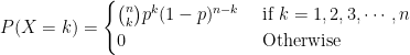
Note: The above PMF can become the PMF for Bernoulli distribution when n = 1.
The mean and variance of a binomial random variable X are given by:
- E(X) = np
- Var(X) = np(1-p)
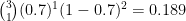
Example 1: Suppose an unfair coin is tossed 3 times with the probability of observing a tail (T) as P(T) = 0.7 and P(H) = 0.3. Let us represent tails by 1 and heads by 0.
Let X is a discrete random variable for the number of heads in each trial. In the entire experiment, there are a total number of 

- Outcome (HHH) is obtained by
leads to x = 3, and probability P(X = 3) =
- Outcomes (HHT), (HTH), (THH) obtained by
leads to x = 2, and probability P(X = 2) =
- Outcomes (HTT), (THT), (TTH) obtained by
leads to x = 1, and probability P(X = 1) =
- Outcome (TTT) obtained by
leads to x = 0, and probability P(X = 0) =


Mean E(X) = 3 * 0.7 = 2.1 and Var(X) = 3 * 0.7 * 0.3 = 0.63
References
- Essentials of Data Science With R Software – 1: Probability and Statistical Inference, By Prof. Shalabh, Dept. of Mathematics and Statistics, IIT Kanpur.
CITE THIS AS:
“Probability and Statistical Inference – Introduction to Bernoulli and Binomial Probability Distributions” From NotePub.io – Publish & Share Note! https://notepub.io/notes/mathematics/statistics/statistical-inference-for-data-science/bernoulli-and-binomial-distributions/
22,415 total views, 1 views today