Essentials of Data Science – Probability and Statistical Inference - Discrete Random Variables

In the previous note on continuous random variables, we have seen what a continuous random variable is and its distribution function. The distribution function is expressed in terms of probability density function (PDF) that helps us to compute the statistical parameters of continuous random variable.

In this note, we will further extend the concept of the random variable and explore discrete random variable and its distribution function. In this case, it is expressed in terms of probability mass function (PMF).

Table of Contents hide

1 Introduction

2 Discrete Random Variable

3 Probability Distribution

3.1 Example 1: Tossing a coin

3.2 Example 2: Tossing two coins

4 Probability Mass Function (PMF)

5 Cumulative Distribution Function (CDF)

5.1 Example 1: Rolling of fair six sided die

5.2 Example 2: Sum of two numbers from two different sets.

6 References

6.1 Share this:

6.2 Like this:

Introduction

Whenever a sample space contains the integer numbers or subset of integer numbers, we express experiment data or sample space using a discrete random variable to model it mathematically.

Further, to extract meaningful information from the discrete random variable, we use the distribution function, and in this case, the distribution function is represented as a probability mass function. However, the cumulative distribution function uses the probability mass function and cumulatively computes the probability values. And outcomes of the distribution function are helpful to understand the random variable properties statistically.

Note: The random variable is a generic term, and it can be a discrete or continuous random variable. In the same way, the distribution function is a generic term, and the probability mass function and probability density function are the distribution functions for discrete and continuous random variables, respectively.

Discrete Random Variable

A random variable X is defined to be discrete if its probability space is either finite or countable, i.e., it takes only a finite or countable number of values. A set V is called a countable if its elements can be listed. It means there is a one-to-one correspondence between the set V and the positive integers.

Let us understand discrete random variables using an example explained in the below paragraph.

Suppose X denotes the random variable as the number of defective components in an electronic device. The device possesses several characteristics, and the random variable X summarises the device only in terms of the number of defects. Further, the possible values of X are integers from zero up to some large value that represents the maximum number of defects that can be found on one of the devices. Furthermore, if this maximum number is enormous, we might assume that the X range is the set of integers from zero to infinity.

Probability Distribution

The probability distribution of a random variable X is a description of the probabilities associated with the possible values of X. For a discrete random variable, the distribution is specified by a list of the possible values along with the probability of each. It is a convenient way to express the probability in terms of a formula.

For example,

If an experiment follows a uniform distribution, we have a predefined probability mass function (PDF) and cumulative distribution function (CDF). And knowing PDF and CDF, we can quickly compute other statistical parameters that are helpful to understand the outcomes of an experiment statistically.

In practice, a random experiment can offen be summarized with a random variable and its distribution. However, the details of the sample space can often be omitted.

Example 1: Tossing a coin

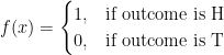
Consider tossing a coin where each trial results in either a head (H) or a tail (T), and each occurs with the same probability, which is 1/2.

The sample space is $\Omega$ = {H,T}.

Let X: number of head.

$f(x) = \begin{cases} 1, & \text{if outcome is H} \\ 0, & \text{if outcome is T} \end{cases}$

Example 2: Tossing two coins

When two coins are tossed, we can observe the outcomes as: $\Omega$ = {HH, HT, TH, TT}. Assuming that each outcome is equally likely then the each occurs with the same probability, which is 1/4.

Let X: Number of heads.

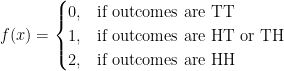
$f(x) = \begin{cases} 0, & \text{if outcomes are TT} \\ 1, & \text{if outcomes are HT or TH} \\ 2, & \text{if outcomes are HH} \end{cases}$ .

It is just a mapping of outcomes to integer values.

Clearly, the sample space of X is the set (0,1,2). We can see that X is a discrete random variable because its space is finite and can be counted.

Suppose we want to find the probability distributation of a random variable X. Using independene and equally likely assumptions for events are as follows:

P(X = 0) = 1/4
P(X=1) = 1/4 + 1/4 = 1/2
P(X=2) = 1/4.

The following depicts the distribution of probability over the elements of range of X.

x	0	1	2
P(X=x)	1/4	1/2	1/4

Probability Distributation

The cumulative distribution are as follows:

$\sum_{x=0} P(X= x) = 1/4$
$\sum_{x \leq 1} P(X= x) = 1/4 + 1/2 = 3/4$
$\sum_{x \leq 2} P(X= x) = 1/4 + 1/2 + 1/4 = 1$

Probability Mass Function (PMF)

The probability distribution of a random variable X is a description of the probabilities associated with the possible values of X. For a discrete random variable, the distribution is specified by a list of the possible values along with the probability of each. However, in some cases, it is convenient to express the probability in terms of a formula.

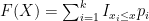
Let X be a discrete random variable which takes k different values. The probability mass function (PMF) of X is given as follows:

$p(X) = P(X=x_i) = p_i \text{ for each } i = 1,2,3, \cdots , k.$

Where $p(X)$ is a probability mass function, $P(X=x_i]$ represents a probability value when a random variable X takes a value called $x_i$ .

It is required that the probabilities $p_i$ satisfy the following conditions:

$0 \leq p_i \leq 1$
$\sum_{i=1}^k p_i = 1$

Cumulative Distribution Function (CDF)

The cumulative distribution function CDF of a discrete random variable as,

$F(X) = \sum_{i=1}^k I_{x_i \leq x} p_i$

Where I is an indicator function defined as follows:

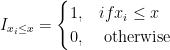
$I_{x_i \leq x} = \begin{cases} 1, & if x_i \leq x \\ 0, & \text{ otherwise } \end{cases}$

The CDF of a discrete variable is always a step function. And knowing the CDF, we can calculate various types of probabilities for discrete random varaibles using it.

Let a. and b be some known constants, then

$P(X \leq a) = F(a)$
$P(X < a) = P(X \leq a) - P(X = a) =F(a) - P(X =a)$
$P(X > a) = 1- P(X \leq a) = 1 - F(a)$
$P(X \geq a) = 1- P(X < a) = 1 - F(a) + P(X = a)$
$P(a \leq X \leq b) = P(X \leq b) - P(X < a) = F(b) - F(a) + P(X = a)$
$P(a < X \leq b) = F(b) - F(a)$
$P(a < X < b) = F(b) - F(a) - P(X=b)$
$P(a \leq X < b) = F(b) - F(a) - P(X=b) + P(X=a)$

Example 1: Rolling of fair six sided die

There are six possible outcomes of rolling a die. Let X be a discrete random variable which is defined as follows: X = Number of dots observed on the upper surface of the die. The six possible outcomes can be as follows.

$X = {x_1=1, x_2=2, x_3=3, x_4=4, x_5=5, x_6=6}$

The PMF is defined as follows:

$p(x) = \begin{cases} 1/6, & \text{if x = 1} \\ 1/6, & \text{if x = 2} \\ 1/6, & \text{if x = 3} \\ 1/6, & \text{if x = 4} \\ 1/6, & \text{if x = 5} \\ 1/6, & \text{if x = 6} \\ 0, & \text{otherwise }\end{cases}$

If we plot the values of $p(x_i) \text{ against } x_i$ , then we will get the following graph. For each value of $x_i$ we will get the probability value of 1/6, which is not true in the case of CDF.

Probability Mass Function: Rolling of fair six sided die — Probability Mass Function: Rolling of fair six-sided die

The CDF is defined as follows:

$F(x) = \begin{cases} 0, & \text{if } -\infty < x < 1 \\ 1/6, & \text{if } 1 \leq x < 2 \\ 1/6, & \text{if } 2 \leq x < 3 \\ 1/6, & \text{if } 3 \leq x < 4 \\ 1/6, & \text{if } 4 \leq x < 5 \\ 1/6, & \text{if } 5 \leq x < 6 \\ 1/6, & \text{if } 6 \leq x < \infty \\ \end{cases}$

CDF gives the cumulative values, suppose we want to find $F(X \leq 2)$ :

$\begin{aligned}F(X \leq 2) & = p(X=1) + p( X= 2) \\ & = 1/6 + 1/6 \\ & = 2/6 = 1/3\end{aligned}$

Cumulative Distribution Function: Rolling of fair six sided die — Cumulative Distribution Function: Rolling of fair six-sided die

Example 2: Sum of two numbers from two different sets.

Suppose m and n are two numbers such that m = 1,2,3 and n = 1,2. Let X be a discrete random variable which is defined as follows: X = All pairs of sum of number from two sets, such as X(m,n) = m + n.

Clearly, there are four possible outcomes that are as follows: (2, 3, 4, 5) from the sample space {(1,1),(1,2),(2,1),(2,2),(3,1),(3,2)}. For example. X(m,n) = X(1,1) = 2, X(1,2) = 3, and so on.

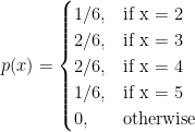
The PMF is defined as follows:

$p(x) = \begin{cases} 1/6, & \text{if x = 2} \\ 2/6, & \text{if x = 3} \\ 2/6, & \text{if x = 4} \\ 1/6, & \text{if x = 5} \\ 0, & \text{otherwise }\end{cases}$

The CDF is defined as follows:

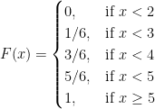
$F(x) = \begin{cases} 0, & \text{if } x < 2 \\ 1/6, & \text{if } x < 3 \\ 3/6, & \text{if } x < 4 \\ 5/6, & \text{if } x < 5 \\ 1, & \text{if } x \geq 5 \end{cases}$

Observe that F is a step function increasing only by jumps. If F is a step function, then the correspoinding random variable is discrete.

Cumulative Distribution Function: Sum of two numbers from two different sets

References

Essentials of Data Science With R Software – 1: Probability and Statistical Inference, By Prof. Shalabh, Dept. of Mathematics and Statistics, IIT Kanpur.

CITE THIS AS:

“Discrete Random Variables” From NotePub.io – Publish & Share Note! https://notepub.io/notes/mathematics/statistics/statistical-inference-for-data-science/discrete-random-variables/

13,487 total views, 2 views today

Essentials of Data Science – Probability and Statistical Inference – Discrete Random Variables

Introduction

Discrete Random Variable