In this note series on Probability and Statistical Inference, we have already seen the importance of probability distributions and their associated probability functions for discrete random variables and continuous random variables. In addition, we have learned to resemble a natural random phenomenon with these probability distributions. These distributions were Degenerate distribution, Uniform distribution, Bernoulli distribution, Binomial distribution, Poisson distribution, Geometric distribution, and Normal distribution.
This note will cover how to approximate various probability distributions of discrete random variables using a continuous random variable probability distribution function.
Need for Normal Approximation
There are various cases where the data sample is huge, and a normal approximation could provide approximately similar results compared to finding results using the actual distribution function. However, there would be certain conditions which must be satisfied.
As a standard normal distribution, computation is tabular based (lookup table), which makes it less computing intensive compared to other distribution functions where we need to solve mathematical equations.
Normal Approximation to the Binomial Distribution
The normal distribution can be used to approximate binomial probabilities for cases where n is large it is because finding 
For example, consider a histogram, where each of the bars represents binomial probabilities. The area of bars can be approximated by the area under the normal density function as normal distribution is continuous. A continuous normal distribution is used to approximate a discrete binomial distribution, and a modification is needed, referred to as a continuity correction. Let us understand the concept behind continuity correction.
Continuity Correction
It is an adjustment that is made when a discrete distribution is approximated by a continuous distribution. In the below example, we try to create a smooth curve from the bars of the histogram. The steps are as follows:
- Mark the midpoints of the bars of the histogram.
- Join them at all the midpoints from a smooth curve.

We can observe that some parts of the bars are excluded, and other parts are included when we draw a smooth curve using the midpoints over the bars of the histogram.
If X is a binomial random variable with parameters n and p, where 
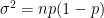

is approximately a standard normal random variable. Note: It is a general formula for standardizing the random variable.
To approximate a binomial probability with a standard normal distribution, a continuity correction is applied as follows:
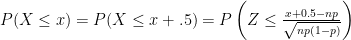
and

The approximation is good when n is large relative to p and (mean) 

References
- Essentials of Data Science With R Software – 1: Probability and Statistical Inference, By Prof. Shalabh, Dept. of Mathematics and Statistics, IIT Kanpur.
CITE THIS AS:
“Probability and Statistical Inference – Introduction to Normal Distribution” From NotePub.io – Publish & Share Note! https://notepub.io/notes/mathematics/statistics/statistical-inference-for-data-science/normal-distribution/
15,233 total views, 1 views today
