Essentials of Data Science – Probability and Statistical Inference - Moments and Variance

In the previous note on the Probability and Statistical Inference, we started a new topic that characterizes the probability distribution of a random variable to get the hidden statistical information about the probability distribution. One of the statistical tools is the expectation of random variables or expectation of the probability distribution of a random variable. We have seen what an expectation is and how to compute the expectation of discrete and continuous random variables.

In this note, we will further explore various tools and techniques that help us characterize the probability distribution of a random variable to get latent information about the random process.

Table of Contents hide

1 Introduction

2 Moments

3 Expectation of Random Variables

3.1 Moment about the origin (Raw Moment)

3.2 Moment about an Arbitrary Point A

3.2.1 Central moments

4 Variance of Random Variables

5 Expectation and Variance of a Random Variable

Introduction

Whenever data comes from some process or experiment, we assume that process can be modeled through probability mass function or probability density function depending on whether the random variable is continuous or discrete. In contrast, suppose there is a curve or graph representing the probability function. By knowing the curve, we can learn more about the probability function of the curve. For example, whether it is symmetric, non-symmetric, humpy, etc.

These statistical tools provide us with the hidden information contained inside the data. The different types of information exist, and these qualities will help us a lot in data science whenever we try to get the actual data without looking into the real data (population data).

The concept of moments is also a particular type of expectation. Moments give enormous information in a quantitative form, which we can’t get or see using graphical or plotting tools when a random variable contains lots of values or large data sets.

Moments

Moments are used to describe different characteristics and features of a probability distribution. These characteristics are: central tendency, disperson, symmetry and peakedness of probability curve. For example:

Symmetry and Peakedness of curve — Skewness of the Curve

So these kinds of information will be computed by Moments which is essential from the analysis and quantitative point of view in Data Science. To understand the Moments, we will first revisit the expectation of random variables concepts, which we studied in the earlier notes of Essential of Data Science.

Expectation of Random Variables

Let X be a continuous random variable with probability density function f(x). Suppose g(X) is a real valued function of X. The expectation of g(X) is defined as:

$E[g(X)] = \int_{-\infty}^{\infty} g(x) f(x) dx$

Provided that $\int |g(x)| f(x) dx < \infty$ .

Let X be a discrete random variable having the probability mass function $P(X=x_i) = p_i$ . Suppose g(X) is a real valued function of X. Thus, X takes the values $x_1, x_2, x_3, \cdots x_k \cdots$ with respective probabilities $p_1, p_2, p_3, \cdots p_k \cdots$ and if the expectation of g(X) exists then,

$\begin{aligned}E[g(X)] &= \sum_{i=1}^{\infty} g(x_i)P(X=x_i) \\ &= \sum_{i=1}^{\infty} g(x_i)p_i \end{aligned}$

Provided that $g(X) = \sum_{i=1}^{\infty} |g(x_i)|p_i < \infty$ .

Moment about the origin (Raw Moment)

Let $g(X) = X^r$ where r is nonnegative integer, then

$E[g(X)] = E(X^r) = \mu^\prime_r$

where $\mu^\prime_r$ is called as $r^{th}$ moment of X about origin or point a zero.

Moment about an Arbitrary Point A

Let $g(X) = (X-A)^r$ where r is nonnegative integer, then $E[g(X)] = E(X - A)^r$ is called as $r^{th}$ moment of X about the point A.

Central moments

When A = $E(X)$ , then $E[(X-A)^r] = E[X - E(X)]^r = \mu^r$ , where, $\mu_r$ is called as $r^{th}$ central moment of X. It is called central moment because moment is measured around the mean.

The moments of variable X about the arithmetic mean ( or sample mean) $\bar{x}$ are called central moments. In general, the $r^{th}$ sample central moment based on observations $x_1, x_2, x_3, \cdots, x_n$ is defined as follows:

$\mu_r$ = $\frac{1}{n} \sum_{i=1}^n (x_i - \bar{x})^r$

Observations:

When r = 0, $\mu_0 = 1$
When r = 1, $\mu_1 = \frac{1}{n} \sum_{i=1}^n (x_i - \bar{x}) = 0$ . It is zero because $\bar{x }$ is a constant (mean value) and $\frac{1}{n} \sum_{i=1}^n x_i = \bar{x}$ only.
When r = 2, $\mu_2 = \frac{1}{n} \sum_{i=1}^n (x_i - \bar{x})^2$ . It is called sample variance.

Variance of Random Variables

In general, when A = $E(X)$ and r = 2, then:

$E[(X-A)^2] = E[X - E(X)]^2 = \mu^2 = \sigma^2$ is called the variance of X.

It computes the variation of X relative to mean value.

The variance of a continuous random variable X is define as:

$\begin{aligned} Var(X) &= E[X - \mu]^2 \\ & = \int_{-\infty}^{\infty} [x - \mu]^2 f(x)dx \end{aligned}$

Where $\mu = E(x)$ .

For a discrete random variable X, the variance of X is defined as:

$\begin{aligned} Var(X) &= E[X - \mu]^2 \\ &= \sum_{i=1}^{n} [x_i - \mu]^2 P(X= x_i) \\ &= \sum_{i=1}^{n} [x_i - \mu]^2 p_i \end{aligned}$

Expectation and Variance of a Random Variable

These are different measures to summarize a probability distribution for a random variable X.

Mean is a measure of the central tendency of the probability distribution.
Variance measures the dispersion or variability in the probability distribution.

It may be possible that two different distributions have the same mean and variance. But, knowing the mean and variance, we can’t predict the probability distribution as these measures do not uniquely identify a probability distribution.

Example 1:

Consider the continuous random variable “waiting time for the train.” Suppose that a train arrives every 20 minutes. Therefore, the waiting time of a particular person is arbitrary and can be any time contained in the interval [0, 20]. The required probability density function is:

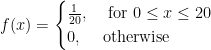
$f(x) = \begin{cases} \frac{1}{20}, & \text{ for } 0 \leq x \leq 20 \\ 0, & \text{otherwise} \end{cases}$

Let X be a continuous random variable for a waiting time for the train. The expected waiting time is as follows:

$\begin{aligned} E(X) &= \int_{-\infty}^{\infty} x f(x) dx \\ &= \int_{0}^{20} x \frac{1}{20} dx \\ &= 10 \end{aligned}$

The variance of a continuous random variable is as follows:

$\begin{aligned} Var(X) &= \int_{-\infty}^{\infty} [x - E(X)^2] f(x) dx \\ &= \int_{0}^{20} (x - 10)^2 \frac{1}{20} dx \\ &= \frac{100}{3} \end{aligned}$

Example 2:

Suppose we roll a dice and rewards are considered in the following ways:

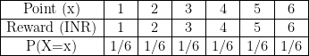
$\begin{array}{|c|c|c|c|c|c|c|} \hline \text{Point (x)} & 1 & 2 & 3 & 4 & 5 & 6 \\ \hline \text{Reward (INR)} & 1 & 2 & 3 & 4 & 5 & 6 \\ \hline \text{P(X=x)} & \text{1/6} & \text{1/6} & \text{1/6} & \text{1/6} & \text{1/6} & \text{1/6} \\ \hline \end{array}$

In this example, Point(x) represents a number that appears on the upper face of the die, and Reward (INR) represents rewards for different values of x. However, each outcome’s probabilities are equally likely, which means anyone occurs with the same probability.

The expected reward means when we play this game a significantly higher number of times, the accumulated rewards would be equal to the expected reward value.

Expected reward, $E(X)$ = Rs. 1 * 1/6 + Rs. 2 * 1/6 + Rs. 3 * 1/6 + Rs. 4 * 1/6 + Rs. 5 * 1/6 + Rs. 6 * 1/6 = Rs. 3.50
$E(X^2) = 1^2 x \frac{1}{6} + 2^2 x \frac{1}{6} + 3^2 x \frac{1}{6} + 4^2 x \frac{1}{6} + 5^2 x \frac{1}{6} + 6^2 x \frac{1}{6} = 91$
$Var(X) = E(X^2) - [E(X)]^2 = 91 - 3.5 \times 3.5 = 78.75$

Standard Deviation

Standard deviation (or standard error) has an advantage that it has the same units as of data, so easy to compare.

For example, if x is in meter, then $s^2$ is in $\text{meter}^2$ which is not so convenient to interpret. On the other hand, if x is in metr, then s is in meter wihch is more covenient to interpret.

Notations to represent standard deviation for sample and population.

Sample Variance is represented as $s^2$ .
Positive square root of $s^2$ is called as standard error.
Population Variance is represented as $\omega^2$ .
Population standard deviation is represented as $\omega$

Variance (or standard deviation) measures how much the observations vary or how the data is concentrated around the arithmetic mean. Standard deviation has its own interpretation and which is represented as follows:

Lower value of variance ( or standard deviation, standard error) indicates that the data is highly concentrated or less scattered around the mean.The lower value of variance is preferable.
Higher value of variance ( or standard deviation, standard error) indicates that the data is less concentrated or highly scattered around the mean.

References

Essentials of Data Science With R Software – 1: Probability and Statistical Inference, By Prof. Shalabh, Dept. of Mathematics and Statistics, IIT Kanpur.

CITE THIS AS:

“Moments and Variance” From NotePub.io – Publish & Share Note! https://notepub.io/notes/mathematics/statistics/statistical-inference-for-data-science/moments-and-variance/

22,183 total views, 1 views today

Essentials of Data Science – Probability and Statistical Inference – Moments and Variance

Introduction

Moments