In this note series on Probability and Statistical Inference, we have already seen the importance of probability distributions and their associated probability functions for discrete random variables. These distributions were Degenerate distribution, Uniform distribution, Bernoulli distribution, Binomial distribution, Poisson distribution, and Geometric distribution. In addition, we have learned to resemble a natural random phenomenon with these probability distributions.
This note will cover probability distributions and their associated probability functions for continuous random variables. At a very first, we will cover the basic intuition behind uniform distribution for continuous random variables and associated measures such as expectation, variance, and moments. Further, we will also cover various similar phenomena following Uniform distribution.
Moreover, using the probability functions of Continuous Uniform Distribution, we can compute expectation, variance, and other quantitative measures of similar phenomenons.
Condition of a Continuous Uniform Distribution
Suppose in a manufacturing plant, a machine part is manufactured. Ideally, all the manufactured parts should be identical. However, due to many causes, such as variations, temperature fluctuations, operator differences, calibrations, cutting tool wear, bearing wear, raw material changes, etc., there can be small variations in the measurements of the same manufactured parts.
Example 1: Let continuous random variable X denotes the current measured in a thin copper wire in milliamperes (mA). Assume that the range of X is [0,20 mA]. The current at every place in the wire is between 0 and 20 mA.
Example 2: The net weight of a packaged chemical compound is between 150 gm and 160 gm.
Example 3: The volume of a shampoo filled into a container is uniformly distributed between 374 and 380 millilitres.
In the above examples, there is a range of values that a random variable takes and there is always a certain kind of variation and randomness exists in these processes.
The measurement is represented as a random variable X and it is reasonable to model the range of possible values of X with an interval of real numbers. The question comes to why these processes are not modelled as discrete random variables. It is because all the processes take uncountable infinite real values within a range. Thus, modelling with continuous random variables is more appropriate.
Continuous Uniform Distribution
A continuous random variable X is said to follow a uniform distribution in the interval [a,b], if its probability density function (PDF) is given by:


We can also write it as 


Usage of Continuous Uniform Distribution
There are many usages of continuous random variables and one of the uses is a generation of random numbers from a given distribution.
Let U be a uniform (0,1) random variable, i.e., 

has distribution function F.
This is called an inverse transformation method. It is helpful in generating the random numbers from the given distributions.
Example 1: Suppose we want to generate a random variable X having distribution function:

If we let 


Hence we can generate such a random variable X by generating a random number U and then setting 
If u = 0.5, 

Example 2: Suppose we want to generate a random number from X which has an exponential distribution with rate 1 with its distribution function 
If we let 


By taking logarithms both side, we will get the following:

Hence we can generate a random number observation from the given exponential distribution by generating a random number U and then setting 
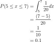
Example 3: Suppose a train arrives at a subway station regularly every 20 minutes. If a passenger arrives at the station without knowing the timetable, then the waiting time to catch the train is uniformly distributed with density

Case 1: The probability of waiting for the train for between 5 and 7 minutes:
Case 2: The probability of waiting for the train for between 2 and 18 minutes:
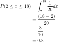
Observe the difference in the probabilities between cases 1 and 2 – 10% vs 80%. It represents a real scenario if we wait for a longer duration then the chances of getting a train are higher.
References
- Essentials of Data Science With R Software – 1: Probability and Statistical Inference, By Prof. Shalabh, Dept. of Mathematics and Statistics, IIT Kanpur.
CITE THIS AS:
“Probability and Statistical Inference – Introduction to Continuous Uniform Distribution” From NotePub.io – Publish & Share Note! https://notepub.io/notes/mathematics/statistics/statistical-inference-for-data-science/continuous-uniform-distribution/
12,375 total views, 1 views today
