In the previous note on the Probability and Statistical Inference, we have seen the the important concept of probability and statistics which are as follows:
- At the very first, we have seen the basic theory of probability and how to model a random phenomenon by satisfying the axioms of probability.
- Further, we explore the random variables and how to model an unexpected phenomenon using random variables and associated probability function based on terms of points and intervals as inputs and find the probability distribution.
- Furthermore, knowing the random phenomenon, probability function, and its distribution, how to apply various measures to characterize the central tendency, dispersion, skewness, and peakedness of the given probability distribution to extract meaning information from it.
In this note and the subsequent notes, we will learn and explore various probability functions and their distributions, which the mathematician already discovered and studied while solving the random phenomenons. These learnings we can use when a given problem matches with a random phenomenon that has already been studied.
Introduction
Our basic assumption is that a probability function can represent every phenomenon. The probability function can be probability mass function or density function depending on the modeling and based on the type of a random phenomenon. Moreover, different kinds of phenomena have different functions that can help us compute probabilities, distributions, and characteristics under specific conditions.
Motivation to read the various probability distributions: Don’t you think that knowing the various random phenomena, their probability function, and characteristics will help solve the problems when the real phenomenon matches the already learned phenomenon or processes.
When we have a probability distribution, we know the probability function. It can be mapped with probability density or probability mass function depending on whether we are working with a discrete or continuous random variable. The selection of random variables and mapping with real-valued functions depends on the random phenomenon. Thus, it shows that when the random phenomenon changes, its associated probability distribution changes.
Need of Probability Distributions
The discrete and continuous probability distributions are widely used for either practical applications or constructing statistical methods.
Suppose we are interested in determining the probability of a particular event. To determination of probabilities depends upon the nature of the study and various prevailing conditions which affect it. The probabilities of different events behave differently.
For example, determining the probability of a head when tossing a coin is different from the probability of rain in the evening. One can guess that some mathematical functions can explain the behavior of probabilities under different situations.
Such functions are called probability distribution functions having special properties and describe how probabilities are distributed under different conditions. The form of such functions depends upon the nature and complexity of the phenomenon under consideration.
We have probability distributions for discrete and continuous random variables. In this and the following notes, we will explore various distributions.
Degenerate Distribution
A random variable X has a degenerate distribution at c, if c is the only possible outcome. The probability mass function (PMF) of X is given by:

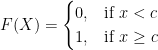
The CDF in such a case is given by:
Further, the mean (expectation) and variance of X are: E(X) = c and Var(X) = 0.
The degenerate distribution indicates that there is only one possible fixed outcome, and therefore, no randomness is involved the examples of degenerate distribution are:
- A two-headed coin.
- Rolling a die whose sides all show the same number.
Discrete Uniform Distribution
Consider a situation where the probability of all the outcomes are the same.
In simple words, it captures those phenomenons where the occurrences of all the outcomes are equally likely.
Examples:
- Tossing a coin where the occurrences of getting head and tail are equally likely.
- Rolling a fair six-sided die where the occurrences of getting any phase of the dice are equally likely.
- Drawing a ball from the box without looking into it, the occurrences of getting any ball are equally likely.
In such situations, the discrete uniform distribution can be used to describe the probabilities and the phenomenon. Moreover, the discrete uniform distribution assumes that all possible outcomes have an equal probability of occurrence.
Probability Mass Function (PMF)
A discrete random variable X with k possible outcomes 
Mean & Variance
If the outcomes are the natural number 

Example 1:
Consider the rolling of a dice. The outcomes 1, 2, 3, 4, 5, and 6 are equiprobabile and 
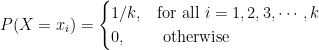
The random variable X is defined as the number of dots observed on the upper surface of the die has a unifrom discrete distribution with PMF:

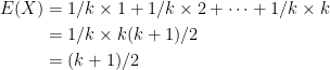
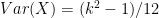
The mean and variance of X are as follows:

References
- Essentials of Data Science With R Software – 1: Probability and Statistical Inference, By Prof. Shalabh, Dept. of Mathematics and Statistics, IIT Kanpur.
- https://www.wikidoc.org/index.php/Degenerate_distribution
CITE THIS AS:
“Probability and Statistical Inference – Introduction to Probability Distributions” From NotePub.io – Publish & Share Note! https://notepub.io/notes/mathematics/statistics/statistical-inference-for-data-science/introduction-to-probability-distributions/
22,420 total views, 1 views today